OpenCV-Mitosis-Detection
Automated Mitosis Detection and Analysis in Histological Images Using OpenCV and Image Processing Techniques
Efim Shliamin
Prerequisites
To run this program, you need to have the following installed:
- Python 3.9 or later
- Miniconda or Anaconda
Installation
Follow these steps to set up your environment and install the necessary packages.
Step 1: Install Miniconda
Download and install Miniconda for your platform from the official Miniconda website.
Step 2: Create a Conda Environment
Open your terminal and create a new Conda environment with Python 3.9:
conda create --name mitosis_env python=3.9
conda activate mitosis_env
Step 3: Install Required Packages
Install the required packages using conda and pip:
conda install numpy matplotlib
pip install imutils opencv-python
Step 4: Add the Conda Environment to Jupyter
To use the Conda environment in Jupyter Notebook, install ipykernel and add the environment:
conda install ipykernel
python -m ipykernel install --user --name=mitosis_env --display-name "Python (mitosis_env)"
Step 5: Run Jupyter Notebook
Start Jupyter Notebook:
jupyter notebook
Usage:
- Place your images in the
mitosis_data_set/directory. - Run the Jupyter Notebook and execute the cells to process the images and display the results.
# Plots are displayed inline in the notebook
%matplotlib inline
import numpy as np
import imutils
import argparse
import cv2
import matplotlib.pyplot as plt
from os import listdir
from os.path import isfile, join
# This program finds all mitoses in all 20 photos with 100% accuracy. Please press "p" to check:
answer = input("'Enter' - display only the results, \n'p' - display the results along with an automatic check:\n")
path = "mitosis_data_set/"
files = [f for f in listdir(path) if isfile(join(path, f))]
correct_solutions = 0 # <- for auto-check
for file in files:
# 1.0 Open image:
file_name = file
img = cv2.imread(path + file_name)
# 2.0 Preprocessing:
rgb_img = cv2.cvtColor(img, cv2.COLOR_BGR2RGB) # for demonstration in plot
hsv_img = cv2.cvtColor(rgb_img, cv2.COLOR_RGB2HSV) # for further segmentation
# 3.0 Segmentation:
# 3.1 Define the color range to detect for brown:
lower_brown = np.array([10, 100, 20])
upper_brown = np.array([20, 255, 200])
# Why these values? It is known that mitoses in these images are recognizable as brownish structures.
# Therefore, the HSV range for BROWN color in openCV is needed here:
# https://stackoverflow.com/questions/46112326/what-is-the-range-of-hsv-values-for-brown-color-in-opencv
# By applying a mask for brown, we select all brown objects in the image:
mask_brown = cv2.inRange(hsv_img, lower_brown, upper_brown)
# 3.2 Apply the mask:
result = cv2.bitwise_and(rgb_img, rgb_img, mask=mask_brown)
# 4.0 Object detection:
# 4.1 The goal of this step is to detect geometric objects in a grayscale image after segmentation:
gray = cv2.cvtColor(result, cv2.COLOR_RGB2GRAY)
# 4.2 Algorithm for detecting geometric structures: edge detection -> Canny filter
# (https://www.uni-ulm.de/fileadmin/website_uni_ulm/mawi.inst.070/funken/bachelorarbeiten/bachelorarbeitBekeJungeEnd.pdf)
edges = cv2.Canny(gray, 100, 250) # The second and third arguments are our minVal and maxVal.
# Why these values?
# a) All edges with an intensity greater than "maxVal" are the sure edges.
# b) All edges with an intensity less than "minVal" are definitely not edges.
# c) The edges between the "maxVal" and "minVal" thresholds are classified as edges only if they are connected to a sure edge, otherwise, they are discarded.
# This ratio is a recommendation from Canny! -> https://docs.opencv.org/3.4/da/d5c/tutorial_canny_detector.html
# So, Canny recommended an upper:lower ratio between 2:1 and 3:1. Hence, the most average value 2.5:1 was chosen
# 4.3 Calculation of suitable features:
# First, we need to perform some morphological transformations (closing & opening).
# We want to close gaps within the edges to make the objects more cohesive
# and facilitate the finding of contours:
kernel = np.ones((5, 5), np.uint8)
closing = cv2.morphologyEx(edges, cv2.MORPH_CLOSE, kernel, iterations=7)
# Then we want to remove some noise:
opening = cv2.morphologyEx(closing, cv2.MORPH_OPEN, kernel, iterations=3)
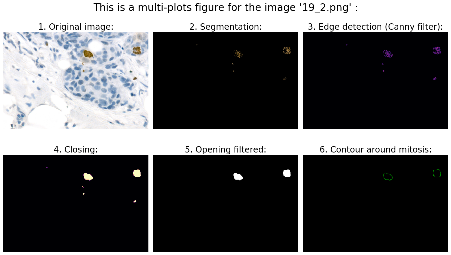
# Why these values? A 5x5 kernel, 7 closing iterations, and 3 opening iterations allow us
# to detect contours of at least 168.5 pixels in size. This is the size
# of the contour found in image '19_2.png' that is not mitosis.
# This means that this configuration is empirically (95% accuracy) quite accurate and sensitive.
# Why?
# Given the image resolution, the nucleus of mammalian cells takes up approximately 41 to 123 pixels.
# Thus, the program is able to recognize contours with an area close to the nucleus of mammalian cells
# at the given image resolution.
# In the next step, we need to eliminate all contours that have too little surface area (<480 pixels, empirically).
# We can now use .findContours and .drawContours
# to retrieve the external contours found by the Canny detection and modified by us ...:
contours, hierarchy = cv2.findContours(opening, cv2.RETR_TREE, cv2.CHAIN_APPROX_SIMPLE)
# Create an empty mask:
mask = np.zeros(opening.shape[:2], dtype=opening.dtype)
# Draw all contours larger than 480 on the mask (see above):
for c in contours:
if cv2.contourArea(c) > 480: # (see above)
x, y, w, h = cv2.boundingRect(c)
cv2.drawContours(mask, [c], 0, (255), -1)
# Apply the mask to the original image:
opening_filtered = cv2.bitwise_and(opening, opening, mask=mask)
# Use .findContours again:
contours_filtered, hierarchy_filtered = cv2.findContours(opening_filtered, cv2.RETR_TREE, cv2.CHAIN_APPROX_SIMPLE)
# ... and draw contour around mitosis on a black background for clarification:
ret, black = cv2.threshold(rgb_img, 255, 255, cv2.THRESH_BINARY)
img_contours = cv2.drawContours(black, contours_filtered, -1, (0, 255, 0), 2)
# 5.0 Analysis:
number_of_objects_in_image = len(contours_filtered)
if answer == "p":
# ---- info + auto-check: ----
file_name_last_char_int = int(file_name[-5])
if number_of_objects_in_image == file_name_last_char_int:
print("Found mitoses in the image " + "'" + file_name + "'" + ":", str(number_of_objects_in_image), "✅")
correct_solutions += 1
else:
print("Found mitoses in the image " + "'" + file_name + "'" + ":", str(number_of_objects_in_image), "❌")
else:
# ------ only info: ------
print("Found mitoses in the image " + "'" + file_name + "'" + ":", str(number_of_objects_in_image))
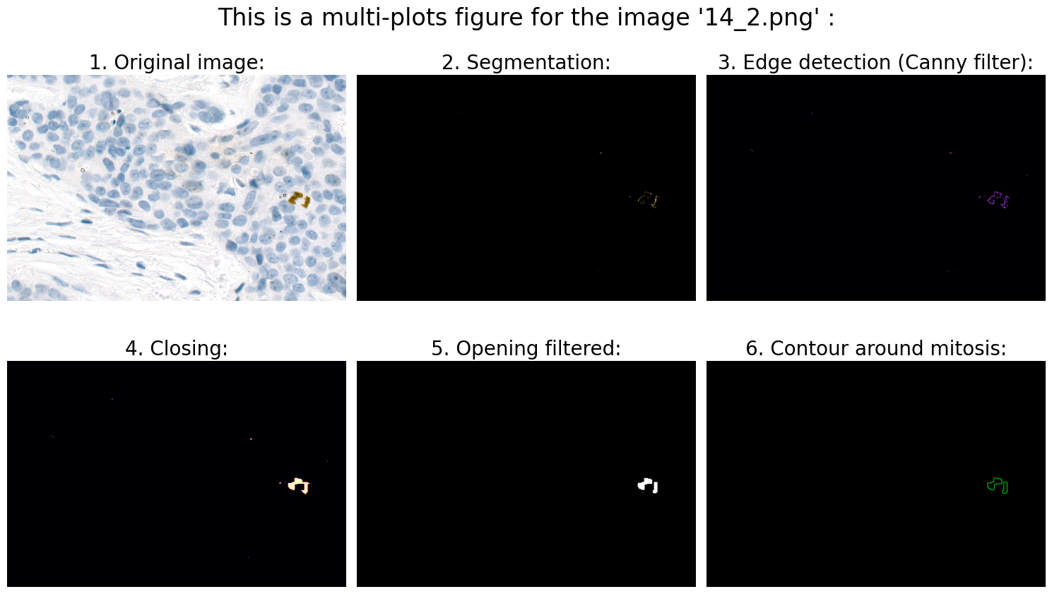
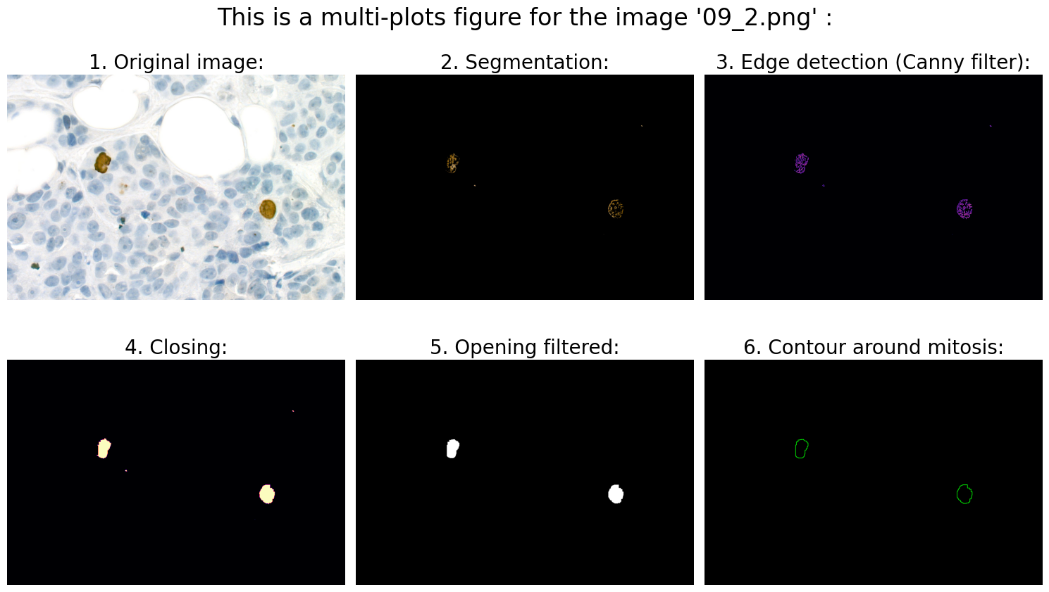
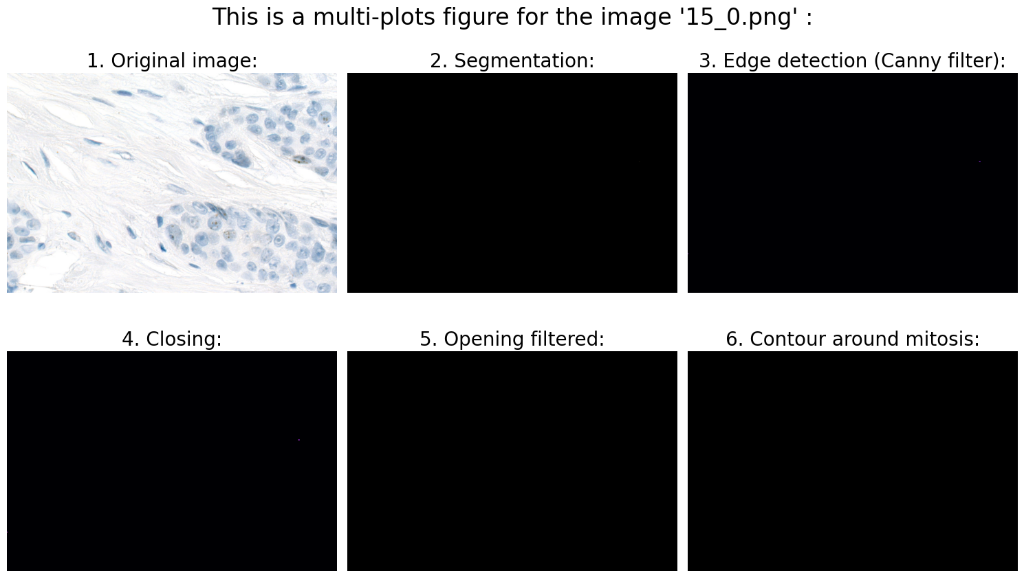
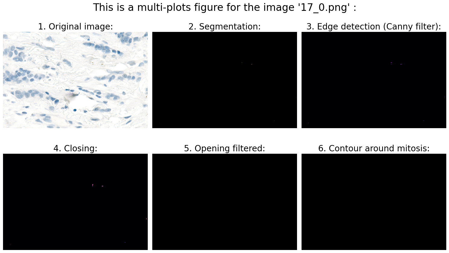
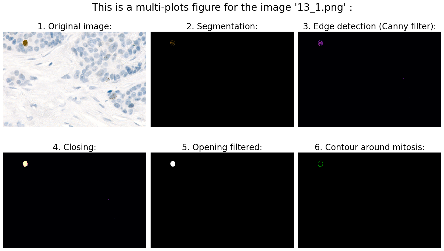
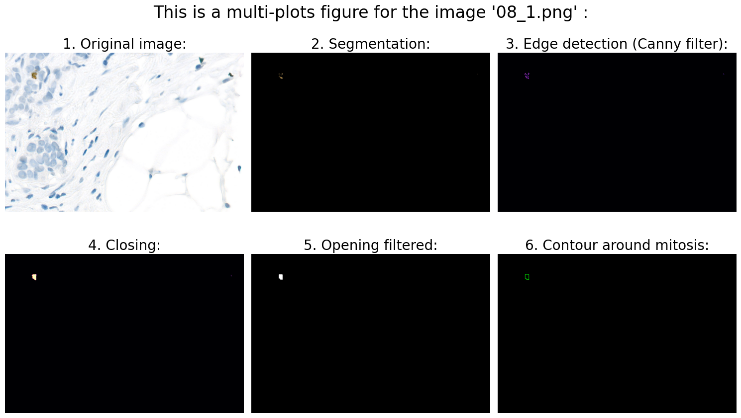
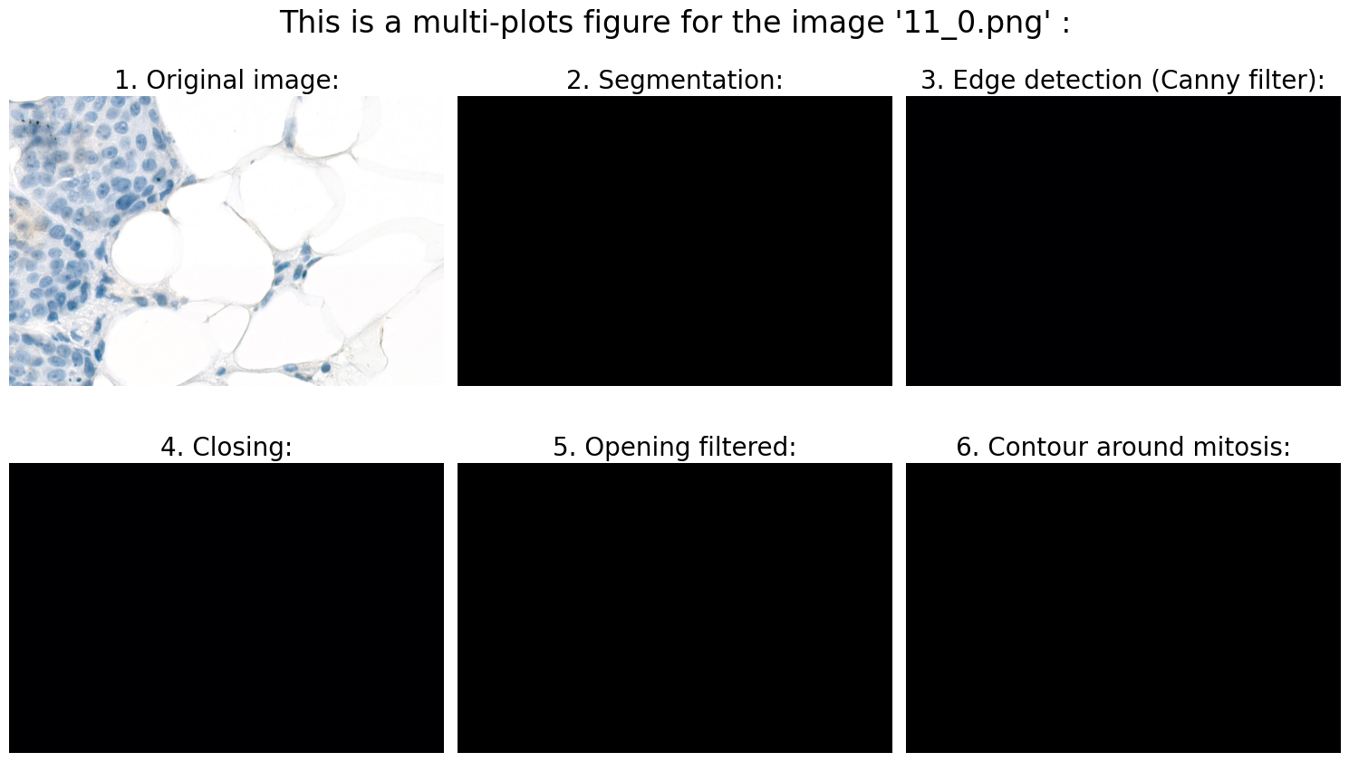
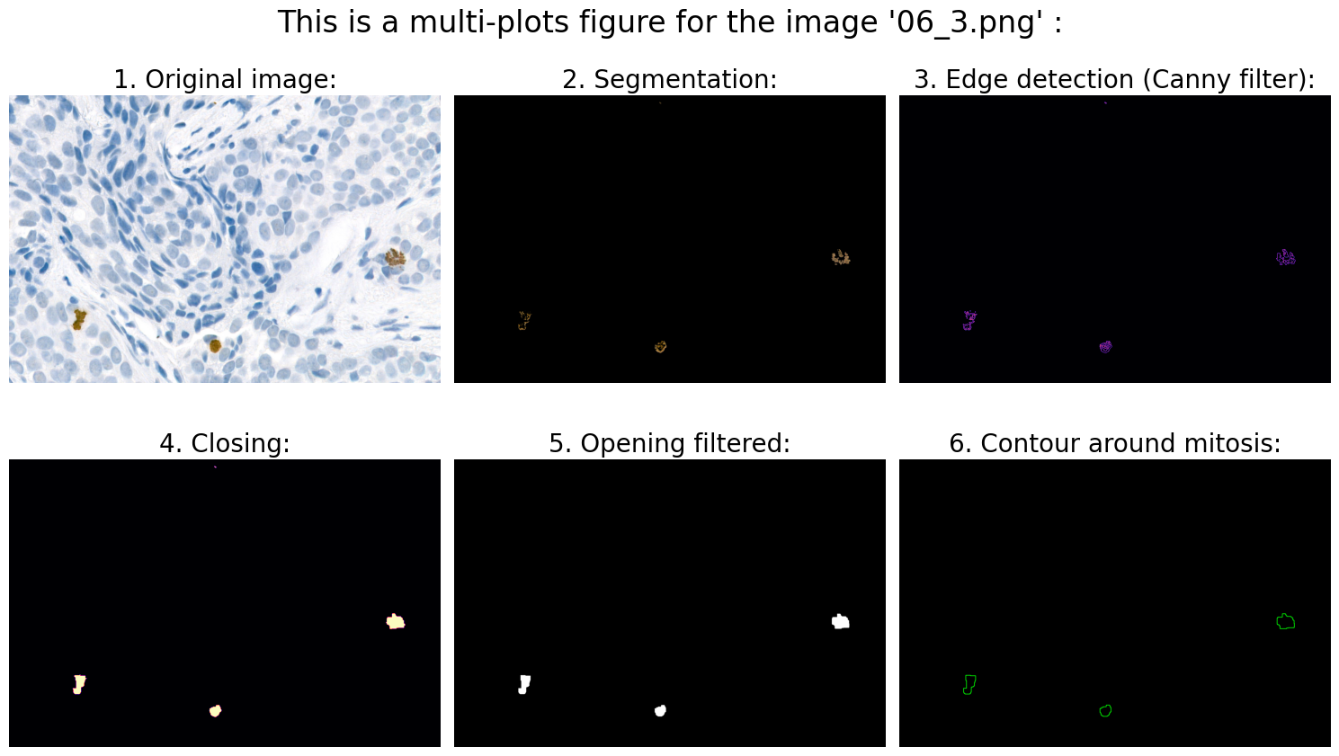
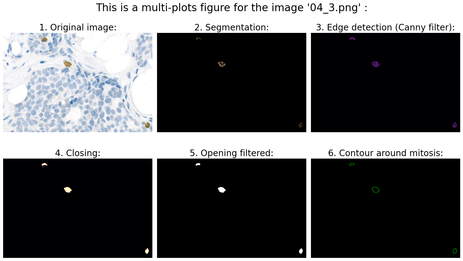
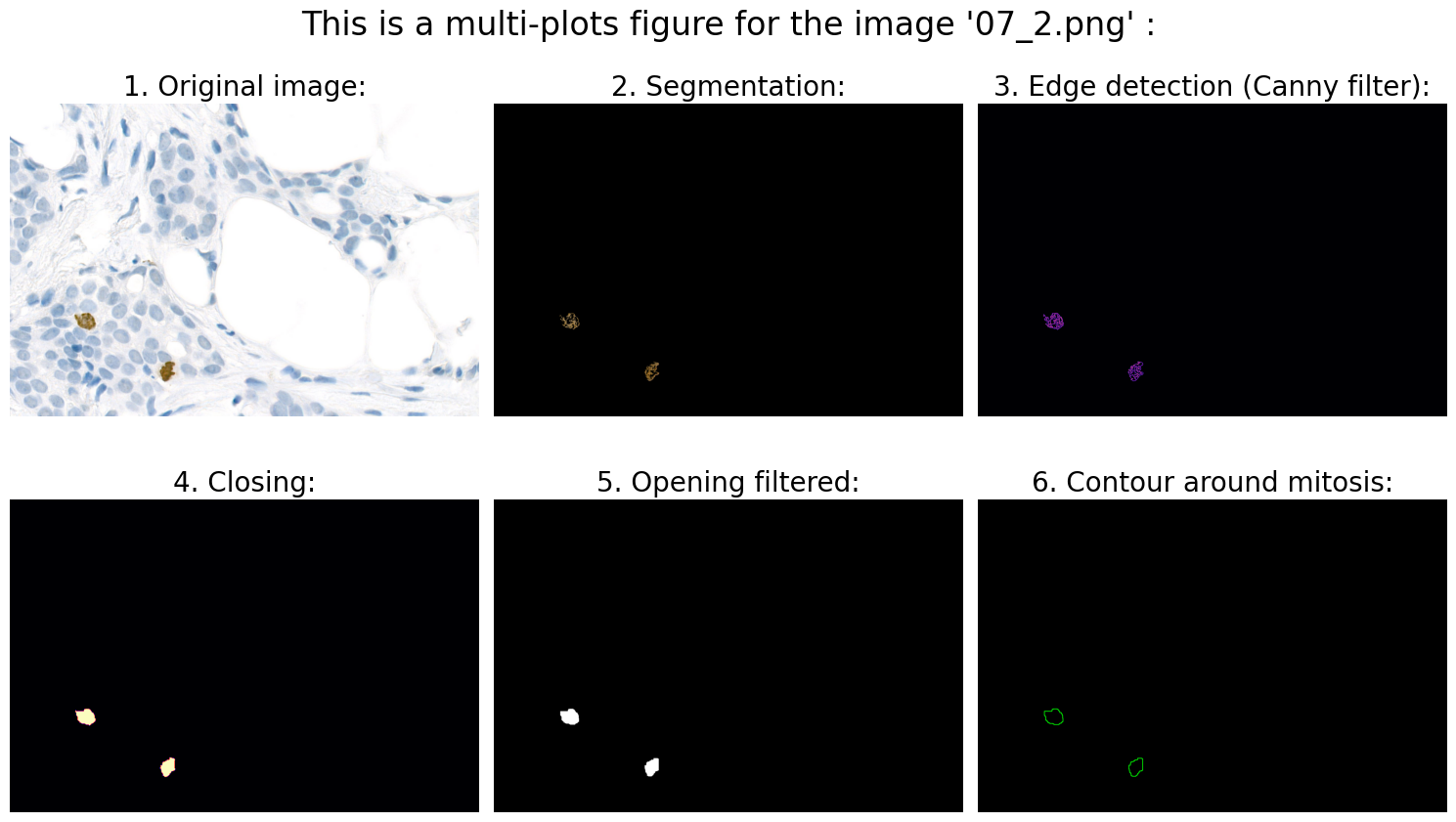
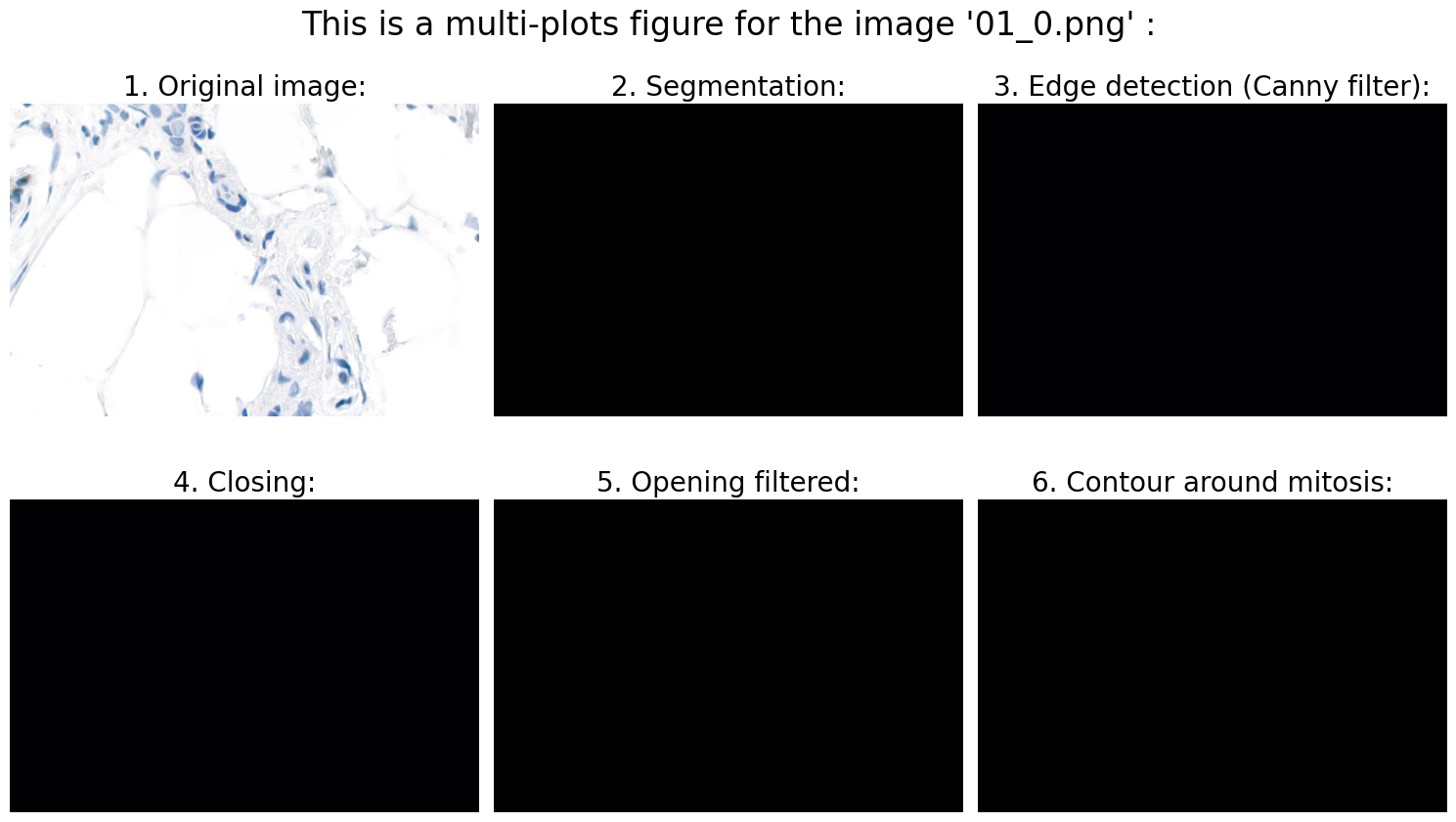
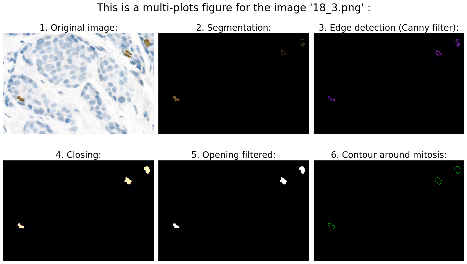
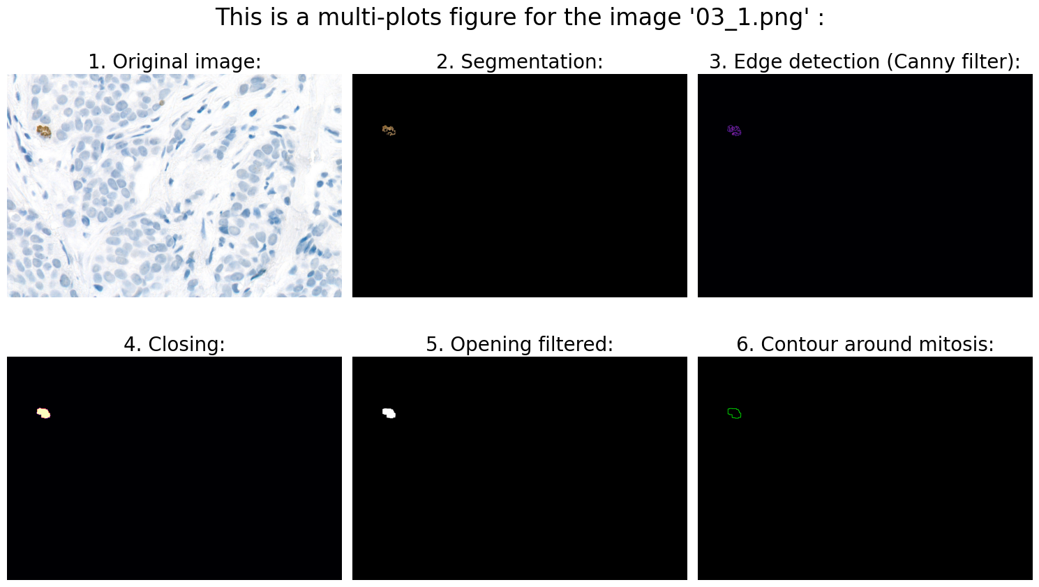
# 6.0 Visualization:
# 6.1 Define fig:
fig_title = "This is a multi-plots figure for the image " + "'" + file_name + "'" + " :"
fig, ((ax1, ax2, ax3), (ax4, ax5, ax6)) = plt.subplots(nrows=2, ncols=3, figsize=(15, 9))
fig.suptitle(fig_title, fontsize=24, y=0.98)
# 6.2 Original image:
ax1.imshow(rgb_img)
ax1.axis('off')
ax1.set_title('1. Original image:', fontsize=20)
# 6.3 Segmentation:
ax2.imshow(result)
ax2.axis('off')
ax2.set_title('2. Segmentation:', fontsize=20)
# 6.4 Edge detection (Canny filter):
ax3.imshow(edges, cmap='magma')
ax3.axis('off')
ax3.set_title('3. Edge detection (Canny filter):', fontsize=20)
# 6.5 Closing:
ax4.imshow(closing, cmap='magma')
ax4.axis('off')
ax4.set_title('4. Closing:', fontsize=20)
# 6.6 Opening filtered:
ax5.imshow(opening_filtered, cmap="gray")
ax5.axis('off')
ax5.set_title('5. Opening filtered:', fontsize=20)
# 6.7 Contour around mitosis:
ax6.imshow(img_contours)
ax6.axis('off')
ax6.set_title('6. Contour around mitosis:', fontsize=20)
# 6.8 Show plt:
fig.subplots_adjust(wspace=0.4, hspace=0.9, top=1.0,
bottom=0.02, left=0.02, right=0.98)
plt.tight_layout()
if answer == "p":
# The accuracy of the result is immediately visible for a large number of images:
total_percentage_of_correct_answers = (correct_solutions / len(files)) * 100
print("")
print("Percentage of correct solutions: ", str(total_percentage_of_correct_answers), "%")
'Enter' - display only the results,
'p' - display the results along with an automatic check:
p
Found mitoses in the image '14_2.png': 2 ✅
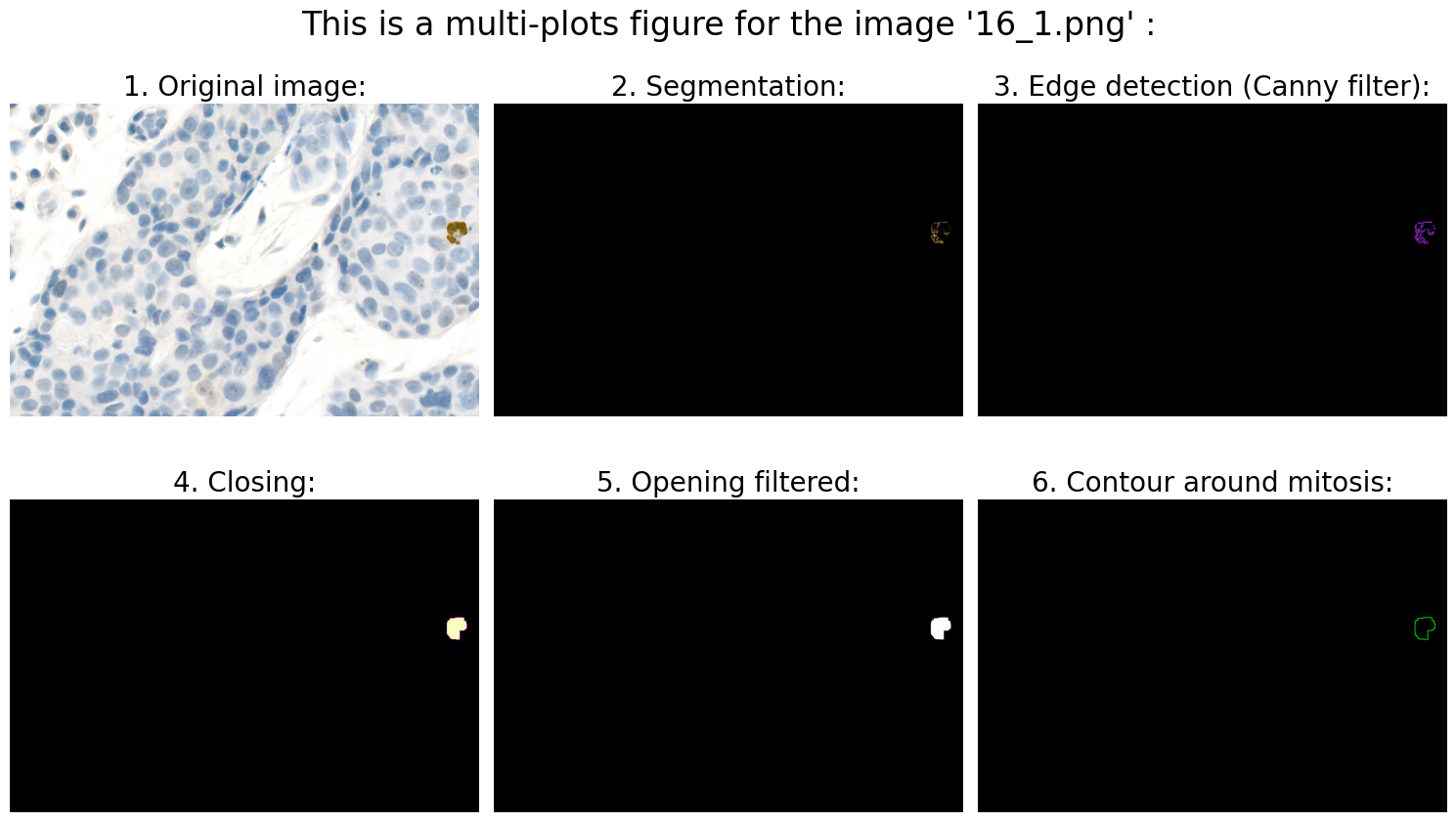
Found mitoses in the image '16_1.png': 1 ✅
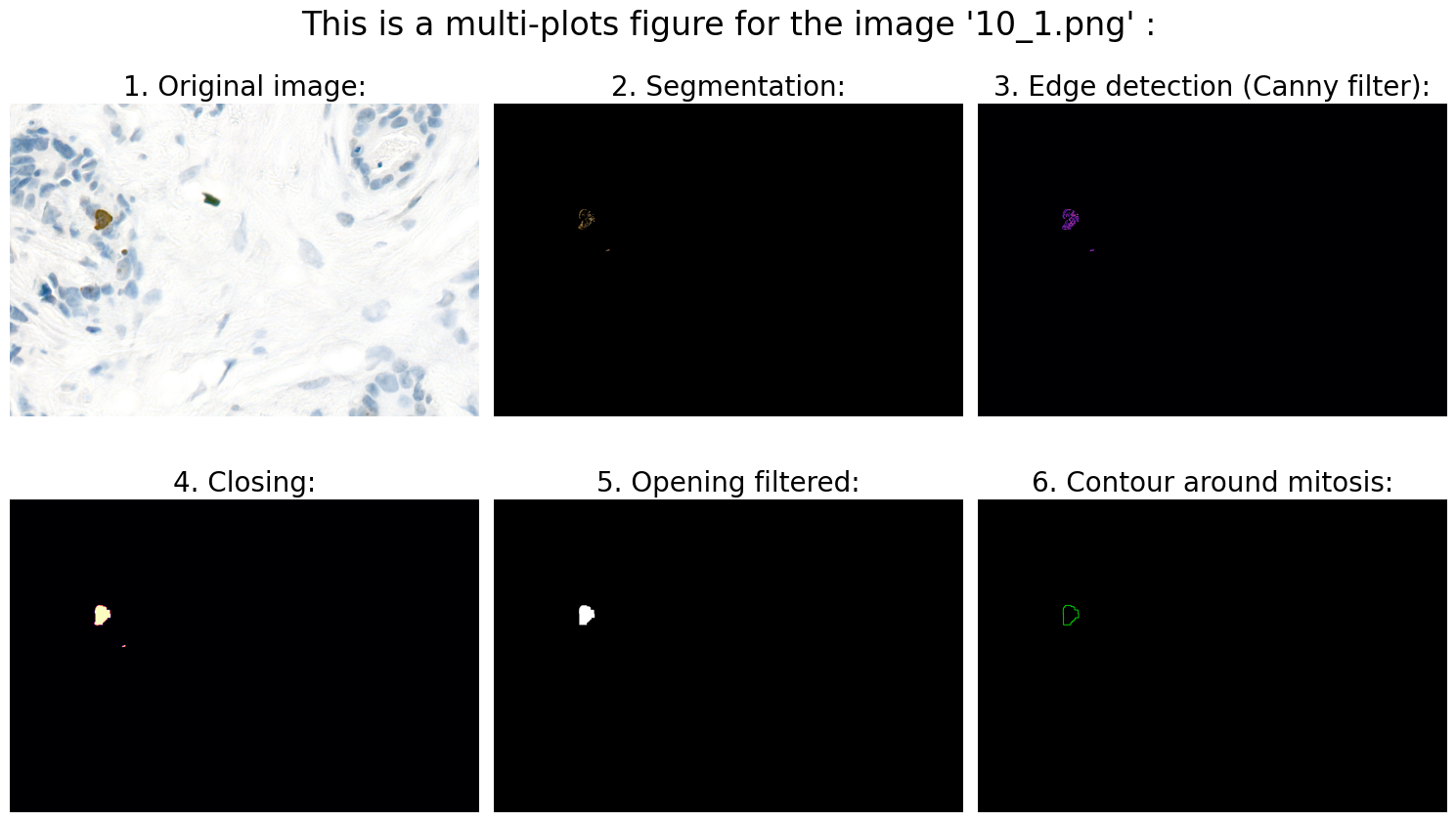
Found mitoses in the image '10_1.png': 1 ✅
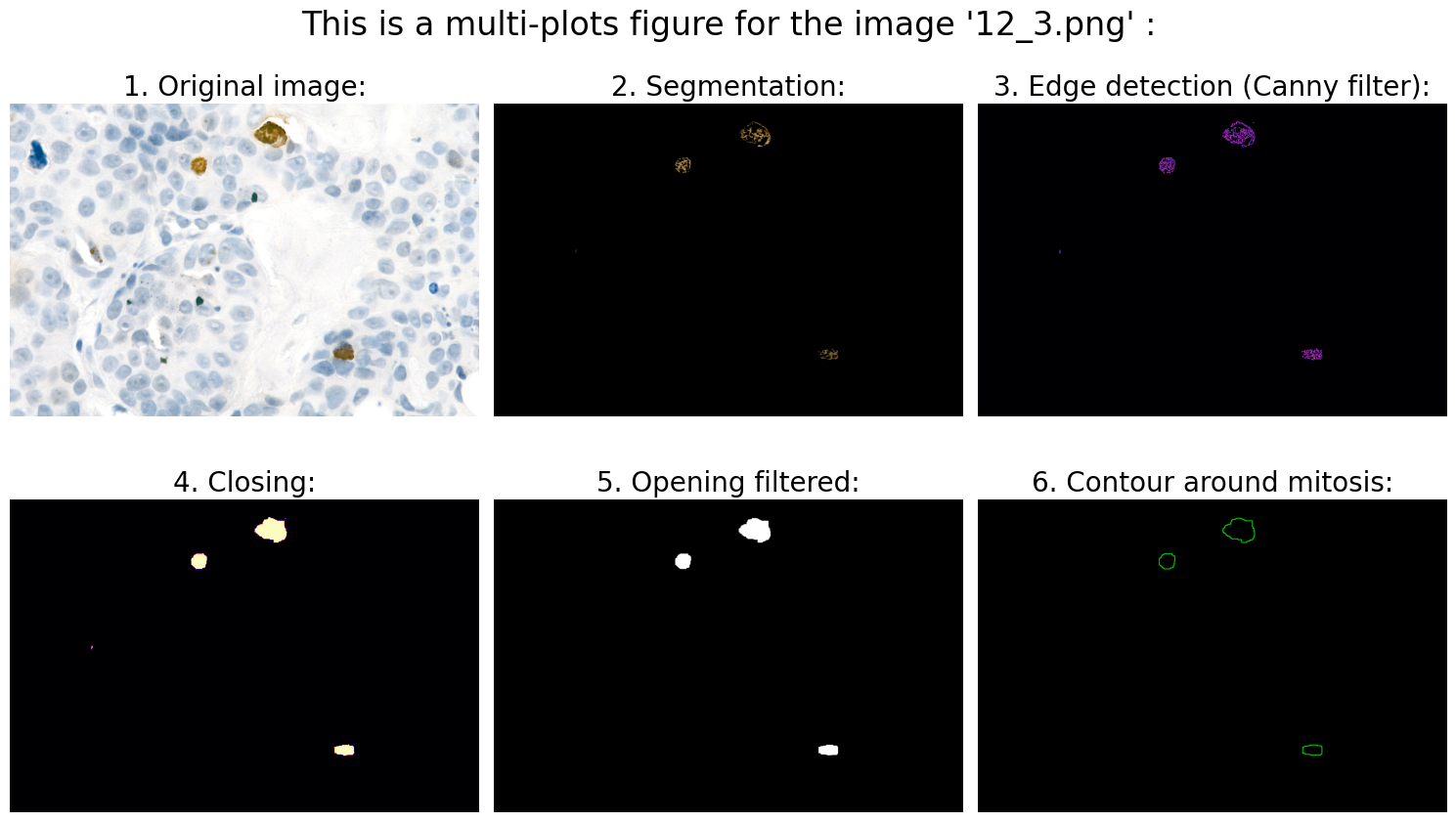
Found mitoses in the image '12_3.png': 3 ✅
Found mitoses in the image '09_2.png': 2 ✅
Found mitoses in the image '15_0.png': 0 ✅
Found mitoses in the image '17_0.png': 0 ✅
Found mitoses in the image '13_1.png': 1 ✅
Found mitoses in the image '08_1.png': 1 ✅
Found mitoses in the image '11_0.png': 0 ✅
Found mitoses in the image '06_3.png': 3 ✅
Found mitoses in the image '04_3.png': 3 ✅
Found mitoses in the image '19_2.png': 2 ✅
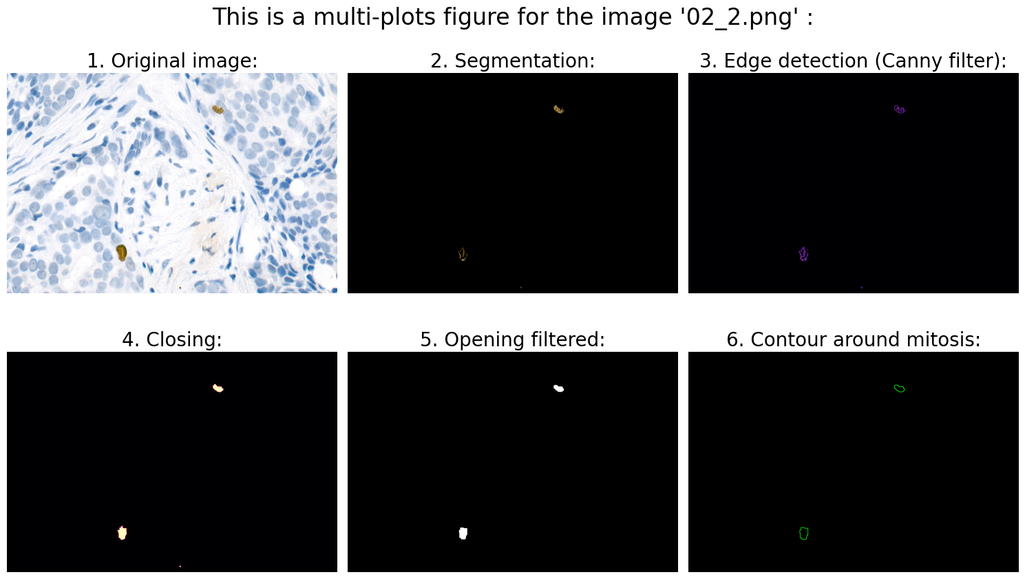
Found mitoses in the image '02_2.png': 2 ✅
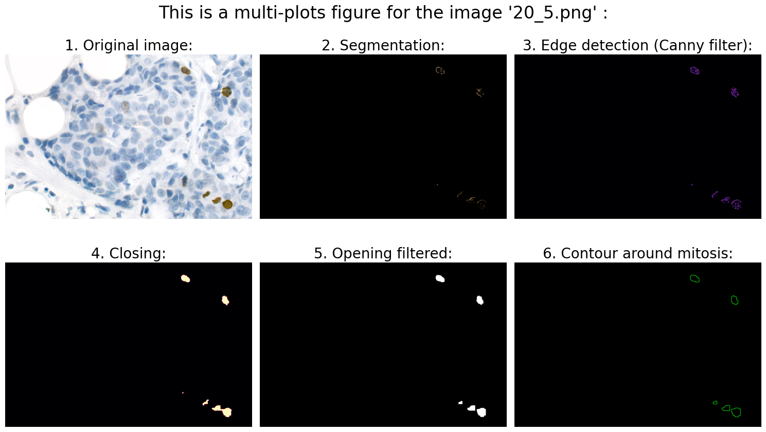
Found mitoses in the image '20_5.png': 5 ✅
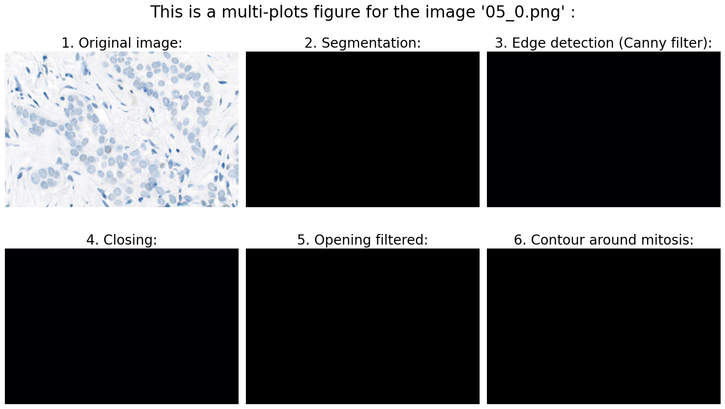
Found mitoses in the image '05_0.png': 0 ✅
Found mitoses in the image '07_2.png': 2 ✅
Found mitoses in the image '01_0.png': 0 ✅
Found mitoses in the image '18_3.png': 3 ✅
Found mitoses in the image '03_1.png': 1 ✅
Percentage of correct solutions: 100.0 %